Detection of Gravitational Waves using Deep Learning

Availability

• Document: here
• Codes: https://github.com/helemnmmm/GW_detection_using_deep_learning

  Introduction

  Gravitational waves (GW) from compact binary coalescences (CBCs) are now routinely detected by ground‑based laser interferometers. The LIGO and Virgo observatories have identified over 90 CBCs during their first three observing runs. Most of these events are binary black hole (BBH) mergers, with only two confirmed binary neutron star (BNS) mergers, and two confirmed neutron star–black hole (NSBH) mergers reported by the end of the third observing run (O3) of the LIGO‑Virgo‑KAGRA collaboration. The first detected BNS merger, GW170817, marked the beginning of a new era of multi‑messenger astronomy, with gravitational waves serving as a crucial messenger. A gamma‑ray burst was serendipitously detected from this merger, along with a kilonova and X‑ray counterpart identified through follow‑up observations. These observations enabled unique measurements of the Hubble constant and provided constraints on the neutron star equation of state. Further observations of BNS mergers could refine constraints on the Hubble constant, address the Hubble tension, and potentially reveal links between BNS mergers and other transient signals, such as fast radio bursts. As interferometer sensitivity improves and new instruments like KAGRA come online, the increasing likelihood of multi‑messenger detections highlights the need for developing new CBC search pipelines.

CBCs are currently detected using five primary search pipelines, four of which employ matched filtering to identify signals. These pipelines use a bank of signal templates with unique intrinsic parameters to cover the mass‑spin parameter space. The templates are cross‑correlated with incoming GW detector data to produce signal‑to‑noise ratio (SNR) time series. In the absence of noise, the highest SNR is achieved by the template whose parameters closely match those of the true signal. Triggers are generated when an SNR threshold is met (e.g., SNR > 4 in one detector). These triggers are then clustered and assigned a significance using a ranking statistic, which typically accounts for the peak SNR, coincident triggers between observing interferometers, and signal consistency tests. Triggers are further evaluated by assigning a false alarm rate (FAR) based on background triggers, and those with sufficiently low FAR are considered GW candidates.

Despite the success of current pipelines in detecting CBCs, exploring new detection methods is worthwhile for several reasons. Firstly, the overall search for CBCs benefits from incorporating multiple pipelines with unique search methods. Unique methods can detect events that might be missed by other pipelines, while joint detections provide stronger evidence that an event is a genuine CBC. Secondly, mitigating non‑Gaussian transient noise artifacts (glitches) remains an ongoing challenge. Glitches can produce high‑SNR triggers, and pipelines must avoid generating alerts based on these while still identifying true CBC signals. As both the detection rate of CBCs and the frequency of instrumental glitches have increased over time, addressing glitches without excluding true signals is becoming increasingly important. A detection method capable of identifying signals while minimizing the impact of glitches, and correctly interpreting signals contaminated by glitches, would be ideal. Given these challenges, deep learning‑based detection methods are a logical avenue for exploration.

Deep learning has already proven useful in enhancing the accuracy and latency of various gravitational wave data analysis tasks. For BBH detection, deep learning has shown promise in achieving sensitivity comparable to matched filtering pipelines in real detector noise. However, applying deep learning to lower‑mass signals like BNS mergers introduces additional challenges. BNS signals are present in detector data for $\mathcal{O}(100~\text{s})$ at current sensitivity, meaning their signal power is significantly more spread out compared to BBH mergers with equivalent SNR. Strain‑based BNS detection methods must either truncate the input window, losing signal power, or make approximations during pre‑processing, which limits sensitivity. Similarly, spectrogram‑based detection methods face analogous limitations. As a result, a deep learning approach for BNS detection that matches the sensitivity of matched filtering pipelines has yet to be demonstrated.

In this work, we investigate the use of a neural network (NN)‑based search pipeline for detecting BNS and BBH mergers in the SNR time series generated by matched filtering. One advantage of detecting signals in the SNR time series is that the CBC signal power is more condensed compared to the strain, which is particularly beneficial for the longer‑duration BNS mergers. Moreover, SNR time series are readily available as data products from matched filtering pipelines, making their online implementation relatively straightforward.

II. Dataset Generation

A. Matched filtering

Matched filtering is a signal processing technique widely used in gravitational wave research, as it provides the optimal method for detecting modeled signals in stationary Gaussian noise. This technique involves cross-correlating a signal template $s$ with incoming detector data $h$, resulting in a signal-to-noise ratio (SNR) time series $\rho(t)$:

B. Template bank generation

We generated our template bank using the LIGO Algorithm Library.

BNS signals:

• IMRPhenomPv2_NRTidalv2 waveform model
• Component masses: $1{-}2.6\,M_\odot$
• Tidal deformability $\Lambda$ sampled within:
  $g_1(m) = a_1 e^{b_1 m},\quad g_2(m) = a_2 e^{b_2 m}$
  with $a_1=6.45\times10^5,\ b_1=-4.386,\ a_2=2.45\times10^5,\ b_2=-6.16$

BBH signals:

• IMRPhenomD waveform model
• Component masses: $5{-}100\,M_\odot$
• Zero spin

Table I. Parameters used to create the template bank.

C. Training dataset construction

• Simulate Gaussian noise (whitened with Welch’s method PSD estimation)
• Random time-shifting (60-80% of time series)
• Training set: 10,000 time series (50% signal+noise)
• Test set: 1,000 samples
• Two augmentation methods compared:
  1. Pre-computed (storage-intensive)
  2. On-the-fly (dynamic during training)

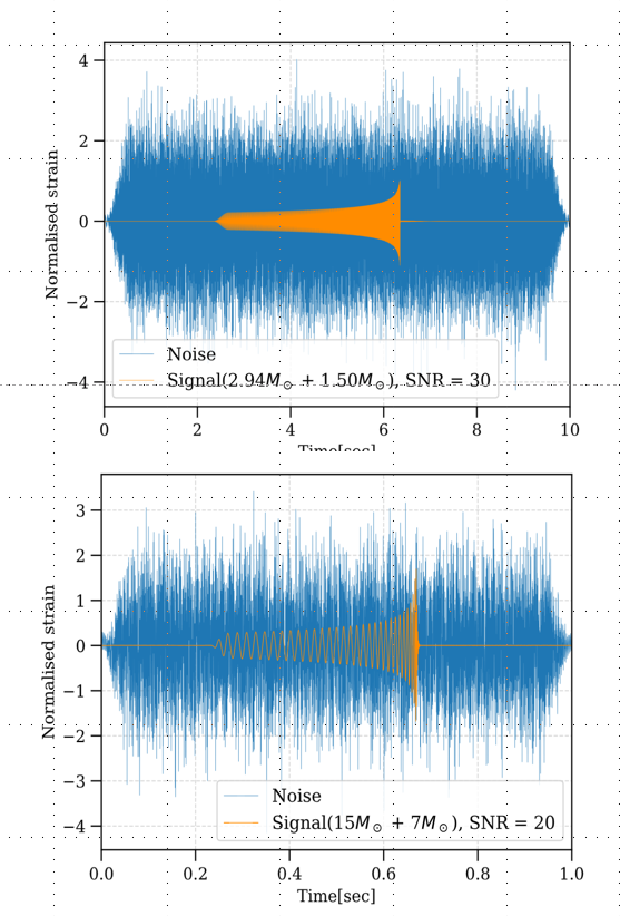
Figure 1. Inserted into simulated LIGO noise are representative signals from binary neutron star (BNS) and binary black hole (BBH) systems. (Upper panel) Presented is a whitened, noise-free temporal sequence representing a gravitational-wave signal from a binary neutron star system with constituent masses of $m_1=2.94M_\odot$ and $m_2=1.5M_\odot$, featuring an optimal signal-to-noise ratio (SNR) of 30. The blue curve illustrates the same gravitational-wave signal superimposed with additive whitened simulated LIGO noise with unit variance. This time series serves as an exemplar within the dataset utilized for training, validation, and testing of the convolutional neural network. (Lower panel) Analogous to the upper panel, this display pertains to a binary black hole gravitational-wave signal characterized by component masses of $m_1=15M_\odot$ and $m_2=7M_\odot$, with an optimal SNR of 20. (Note: $\Lambda = 0$ for black holes.)

III. The Neural Network

A. Model Architecture

We implement two classes of models:

CNN

• 3 convolutional layers (filters: 16, 32, 64, 128) with ELU activations, batch-norm, pooling
• 2 dense layers (64, 2) with dropout
• Softmax output → sigmoid
• Custom scaling layer (÷4 before sigmoid) to avoid 32-bit rounding

Table II. Architecture of the CNN

ResNet (50, 101, 152 layers)

• Standard residual blocks
  • Configurations: [3,4,6,3], [3,4,23,3], [3,8,36,3]
• AvgPool → Flatten → 3 dense layers with dropout → sigmoid

Table III. Architecture of ResNet

B. Training

• Framework: PyTorch
• Optimizer: Adam with AMSGrad, initial learning rate = 0.001
• Batch sizes: 16 (BBH), 8 (BNS) on NVIDIA RTX 4090
• Loss: Sparse categorical cross-entropy

IV. Results

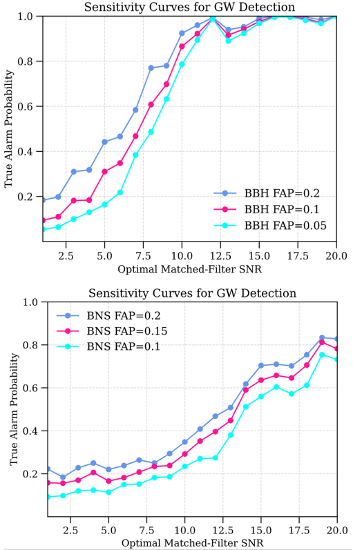
Figure 2. Sensitivity vs. optimal SNR for fixed false alarm probabilities, for BBH (top) and BNS (bottom).

• ROC curves show higher sensitivity for BBH than BNS at equal false alarm probability (FAP).
• CNN reaches maximal sensitivity for BBH at SNR = 10, FAP ≥ 0.1, but fails to saturate for BNS even at SNR = 30.
• On‑the‑fly augmentation (Method 2) converges faster and uses far less storage than Method 1, with only marginal sensitivity loss.
• Model comparison: ResNet architectures outperform CNN, with ResNet101 providing the best sensitivity at low FAP, at the cost of higher computational complexity.

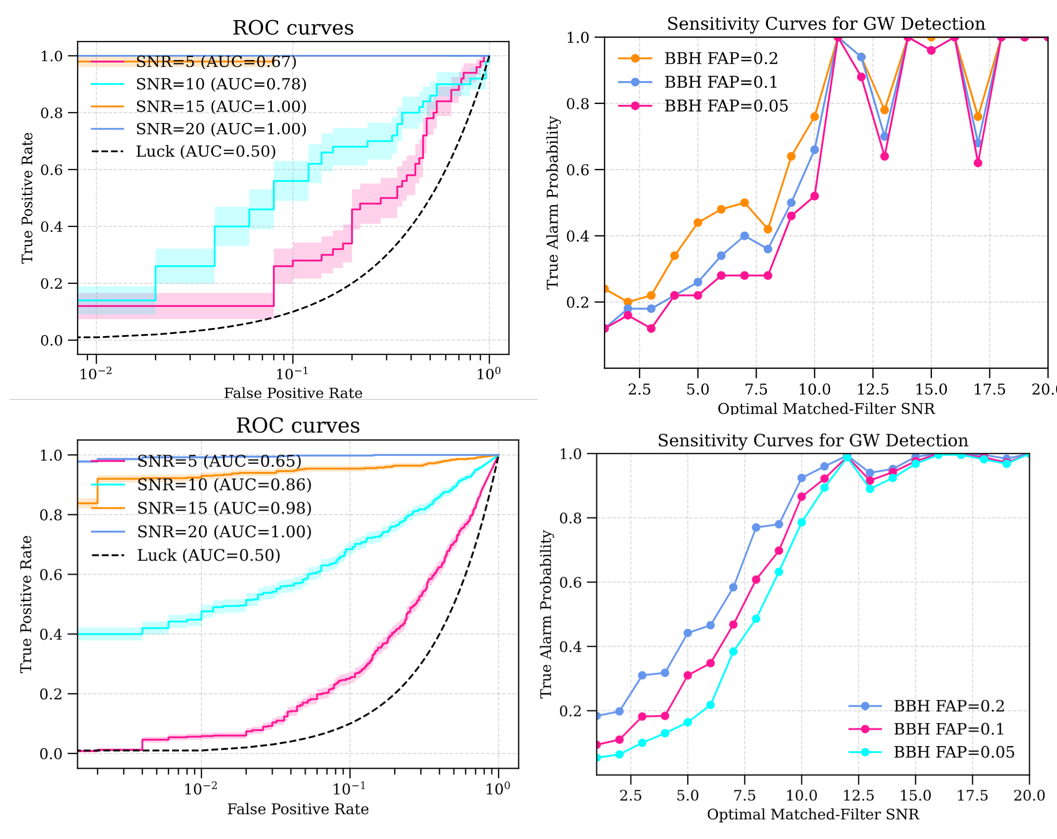
Figure 3. Comparison of data augmentation methods for BBH detection using CNN: Method 1 (top) vs. Method 2 (bottom).

Figure 4. Model comparison (CNN vs. ResNet50 vs. ResNet101) sensitivity curves.

V. Summary and Discussion

In this study, we employ deep learning techniques for gravitational wave (GW) detection tasks, illustrating their potential to attain high sensitivity and robustness in identifying signals from binary black hole (BBH) and binary neutron star (BNS) mergers. We assess the performance of neural networks using CNN, ResNet50, ResNet101, and ResNet152 architectures, comparing their sensitivity curves across various false alarm probabilities (FAPs) and signal-to-noise ratios (SNRs). Additionally, through the utilization of on-the-fly data augmentation and analysis via receiver operating characteristic (ROC) curves, this work offers insights into the balance between computational efficiency and detection efficacy.

The training dataset was carefully assembled to include 5000 samples of both signal-plus-noise and pure noise, maintaining consistent SNR values of 20 for BBH signals and 30 for BNS signals. This configuration facilitated the exposure of the network to a diverse array of samples, promoting generalization. Meanwhile, the testing dataset contained 1,000 samples and was specifically designed to evaluate the model’s proficiency in accurately classifying previously unseen data. Although this configuration represents a substantial advancement towards effective GW detection, the relatively small dataset, particularly regarding BNS signals, seems to have restricted the models’ efficacy. This limitation is most apparent in the less-than-optimal sensitivity observed for BNS detections, underscoring the necessity for additional data augmentation or alternative strategies to improve the representation of BNS signals in the training set.

The empirical ROC curves developed in this research demonstrate that the models attained superior TAPs for BBH signals relative to BNS signals at analogous FAPs. For instance, the CNN model achieves peak sensitivity for BBH signals at an optimal SNR of 10 when FAP $\geq 0.1$. Nonetheless, the model fails to attain a comparable maximum sensitivity for BNS signals, even when the SNR is optimally set at 30. This gap highlights the difficulty in detecting BNS signals, potentially due to their inadequate representation in the training dataset and the inherent disparities in waveform characteristics between BBH and BNS mergers.

It is also notable that at lower SNRs, the TAP for BNS signals remains similar for a range of optimal SNR values (e.g., SNR = 14 and SNR = 18). This implies that the network’s sensitivity does not significantly improve with increasing SNR under certain conditions, pointing to potential limitations in the network’s feature extraction capabilities or the quality of the training data. These findings align with previous works, such as Krastev (2020), which report comparable challenges in detecting BNS signals in simulated Gaussian noise.

Integrating on-the-fly data augmentation markedly enhanced training efficiency and diminished computational overhead relative to conventional pre-computed data generation techniques. Although Method 1 (traditional augmentation) yields slightly superior area under the curve (AUC) scores and sensitivity at fixed False Alarm Probabilities (FAPs) because of its comprehensive feature space coverage, it incurs considerable computational and storage requirements. In contrast, Method 2 (on-the-fly augmentation) dynamically generates augmented data during training, resulting in faster convergence and competitive performance, especially under reduced SNR conditions. The trade-off between efficiency and performance is critical for resource-constrained environments. The results indicate that Method 2 is a compelling alternative for scenarios where computational resources or storage capacity are limited. Additionally, its ability to maintain competitive sensitivity at higher SNR levels makes it a viable choice for real-time GW detection applications. These observations highlight the importance of selecting appropriate data augmentation techniques to balance computational requirements and model performance.

The sensitivity curves for CNN, ResNet50, ResNet101 and ResNet152 architectures reveal notable differences in their ability to detect GW signals. While all three models demonstrate reasonable sensitivity improvements with increasing SNR, the ResNet architectures consistently outperform the CNN, particularly at lower FAPs. ResNet50 and ResNet101 leverage their deeper architectures and residual connections to enhance feature representation and mitigate vanishing gradient issues, resulting in higher TAPs at fixed FAPs. However, the additional depth of ResNet101 does not always translate to significant performance gains compared to ResNet50, particularly when using traditional data augmentation methods (Method 1). This observation suggests that the marginal benefits of increased depth may diminish beyond a certain point, especially when computational complexity and training time are considered. On the other hand, when employing on-the-fly data augmentation (Method 2), ResNet101 achieves optimal sensitivity, highlighting the synergy between advanced architectures and efficient data augmentation strategies.

Despite the promising results, several challenges and limitations warrant further investigation:

• Dataset Quantity and Diversity:
  The limited size and diversity of the training dataset, particularly for BNS signals, constrain the models’ ability to generalize. Future studies should focus on generating larger and more diverse datasets, potentially incorporating real LIGO data to enhance the realism and variability of training samples.

• BNS Signal Detection:
  The suboptimal performance of the models in detecting BNS signals raises questions about their ability to capture the unique features of these waveforms. Investigating alternative network architectures or feature extraction techniques tailored to BNS signals could improve sensitivity.

• SNR Effects:
  The sensitivity analyses indicate that the models’ performance varies significantly with SNR. Further studies are needed to explore the relationship between SNR and detection accuracy, including adjustments to network hyperparameters and training strategies to optimize performance across a broader SNR range.

• Model Optimization:
  While ResNet101 achieves the highest sensitivity, its increased computational complexity poses challenges for real-time applications. Exploring lightweight architectures or pruning techniques could help achieve a balance between performance and efficiency.

• Combined Detection of BBH and BNS Signals:
  Integrating BBH and BNS detection into a unified framework could streamline GW detection workflows and enhance overall efficiency. Developing models capable of distinguishing between these classes while maintaining high sensitivity is an important avenue for future research.

This study demonstrates the potential of deep learning approaches for GW detection, leveraging CNN and ResNet architectures to identify signals from BBH and BNS mergers. The analysis of sensitivity curves and ROC metrics reveals that while ResNet-based models outperform CNNs, their performance for BNS signals remains suboptimal, primarily due to dataset limitations. On-the-fly data augmentation emerges as a promising technique to enhance training efficiency and maintain competitive performance, particularly under reduced SNR conditions.

The findings underscore the importance of dataset quality, network architecture, and data augmentation methods in achieving robust GW detection. Future work should focus on addressing the challenges of dataset diversity, BNS signal detection, and model optimization, with a particular emphasis on integrating real LIGO data and exploring unified frameworks for detecting BBH and BNS signals. These efforts will contribute to the development of scalable and efficient deep learning-based GW detection systems, paving the way for advancements in astrophysical research and multi-messenger astronomy.

<!--
  See https://www.debugbear.com/blog/responsive-images#w-descriptors-and-the-sizes-attribute and
  https://developer.mozilla.org/en-US/docs/Learn/HTML/Multimedia_and_embedding/Responsive_images for info on defining 'sizes' for responsive images
-->

  
    <source
      class="responsive-img-srcset"
      
        srcset="/assets/img/1-480.webp 480w,/assets/img/1-800.webp 800w,/assets/img/1-1400.webp 1400w,"
        type="image/webp"
      
      
        sizes="95vw"
      
    >
  

<img
  src="/assets/img/1.jpg"
  
    class="img-fluid rounded z-depth-1"
  
  
    width="100%"
  
  
    height="auto"
  
  
  
  
    title="example image"
  
  
  
    loading="eager"
  
  onerror="this.onerror=null; $('.responsive-img-srcset').remove();"
>

</picture>

</figure>

</div>
<div class="col-sm mt-3 mt-md-0">

</div>
<div class="col-sm mt-3 mt-md-0">

</div>

</div>

–>

<!--
  See https://www.debugbear.com/blog/responsive-images#w-descriptors-and-the-sizes-attribute and
  https://developer.mozilla.org/en-US/docs/Learn/HTML/Multimedia_and_embedding/Responsive_images for info on defining 'sizes' for responsive images
-->

  
    <source
      class="responsive-img-srcset"
      
        srcset="/assets/img/6-480.webp 480w,/assets/img/6-800.webp 800w,/assets/img/6-1400.webp 1400w,"
        type="image/webp"
      
      
        sizes="95vw"
      
    >
  

<img
  src="/assets/img/6.jpg"
  
    class="img-fluid rounded z-depth-1"
  
  
    width="100%"
  
  
    height="auto"
  
  
  
  
    title="example image"
  
  
  
    loading="lazy"
  
  onerror="this.onerror=null; $('.responsive-img-srcset').remove();"
>

</picture>

</figure>

</div>
<div class="col-sm-4 mt-3 mt-md-0">

</div>

</div>

–>